Hey there,
I recently started to attend a artificial intelligence lecture (a real course, not online) and we have gotten a small intro to NetLogo yesterday. Although I'm not a real fan of it (mainly because I was tortured with LOGO as a kid, you don't know how painful it is if you already know C++), I liked the idea of plotting agents and scripting all kinds of logic in a compressed way.
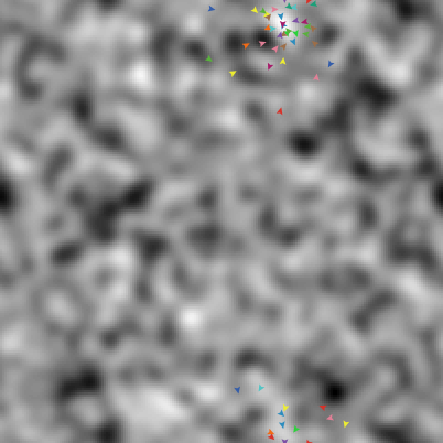
So I used to came across an example in their modules library called "Particle Swarm Optimization" (PSO), which was really amazing. I can give you a small picture of it:
 |
| Particle Swarm Optimization plot Source |
You can see a lot of colored particles (or agents) and a terrain that is greyscaled according to its height. Your job is to find a pretty good minimum (whitened areas) in this terrain via swarm intelligence.
A short summary is, that if you have a function and want to minimize the cost by a given parameter set "Theta", you can use the PSO algorithm to find a good minimum of your function. You can compare this for example with Gradient Descent or Conjugate Gradient, but there is a subtle difference between them, for PSO no differentiable function is needed.
Intuition
Of course I will provide you with the basic intuition of this algorithm. So I told that there is a certain number of agents in this algorithm. They are initialized uniformly distributed in our search space, ideally you want to fill the map to get a good spread of your agents so your chance is higher to find a global minimum.
For a fixed number of iterations, you are going to change the position of each particle randomized with a weight on three objectives which are parameters of this meta-optimizer.
- Alpha (in literature also called φp / Phi_personal) is the weight of an agent following its personal memory (based on prior found minimas)
- Beta (in literature also called φg / Phi_global) is the weight of an agent following the global memory of the swarm (based on the currently best minimum from the swarm)
- Phi (in literature also called ω / Omega) is the inertia/velocity of an agent.
From the parameters you can tell that each particle has its own memory (the best personal found solution), also there is a swarm memory, which basically is just a record of the currently best found solution from all particles.
Math
To understand the weighted formula of the movement of the particles, we have to have a look at the formula:
 |
| Formula to calculate the new position of a particle, based on the current position "v" |
Algorithm
The algorithm is quite easy, because there is some really good pseudo code on Wikipedia.
However here is my small summary of it:
- Initialize...
- the particle positions to some random positions in our search space
- the memorys of the agents and the swarm memory
- In each iteration until we haven't hit our maximum iterations do...
- loop over all particles
- calculate the new position of a particle
- check the cost of this position, if its smaller than the particles memory then update, do the same update with the global memory if its smaller.
- Profit!
This is a nice and easy algorithm. To further visualize it, I have found a very good youtube video about it, implemented with MatLab: http://www.youtube.com/watch?v=bbbUwyMr1W8
There you can see the movement of the particles very well for a number of functions.
In Java
Of course I have done this in Java with my math library. So let's dive into my normal testcase of the function

Which is a good testcase, because it is convex so it has a global minimum which can be good tested.
A nice looking plot of it:
 |
| Convex function f(x,y) = x^2 + y^2 |
Let's sneak into the Java code:
    DoubleVector start = new DenseDoubleVector(new double[] { 2, 5 });

    // our function is f(x,y) = x^2+y^2
    CostFunction inlineFunction = new CostFunction() {
      @Override
      public Tuple<Double, DoubleVector> evaluateCost(DoubleVector input) {

        double cost = Math.pow(input.get(0), 2) + Math.pow(input.get(1), 2);
        return new Tuple<Double, DoubleVector>(cost, null);
      }
    };

    DoubleVector theta = ParticleSwarmOptimization.minimizeFunction(
        inlineFunction, start, 1000, 0.1, 0.2, 0.4, 100, false);
    // retrieve the optimal parameters from theta
We run 1000 particles for 100 iterations, with a weight of 0.1 to the personal best solution, 0.2 to the swarm solution and 0.4 for its own exploration. Basically this was the usage of the algorithm, you can see that we don't need a gradient in this computation (it is nulled). Theta in this case should contain a value close to zero.Of course you can find the source code here:
https://github.com/thomasjungblut/thomasjungblut-common/blob/master/src/de/jungblut/math/minimize/ParticleSwarmOptimization.java
And the testcase above here:
https://github.com/thomasjungblut/thomasjungblut-common/blob/master/test/de/jungblut/math/minimize/ParticleSwarmOptimizationTest.java
And BTW, I just trained a XOR neural network with a single hidden layer with it. This is a very very cool algorithm ;)
A small parameterization tip is to set alpha to 2.8 so it does not fall into local minimas too fast (beta was 0.2 and phi 0.4).
You can have a look how it works in my testcase of the MultiLayerPerceptron:
https://github.com/thomasjungblut/thomasjungblut-common/blob/master/test/de/jungblut/classification/nn/MultiLayerPerceptronTest.java#L40