Hey all,
been a very long time since my last post. I was very busy with
Apache Hama, we have graduated from the Apache incubator and call us now a top level project and of course made another release 0.5.0. I think this was just the beginning of a rising open source project and I am really excited to be a part of it.
However, responsibility comes with spending a lot of time. Time is always sparse, especially if you are young and have a lot of stuff to do.
So blog posts like this will be very sparse in the future, but today it should not matter and I will tell you about a semi-supervised learning algorithm with the very phonetic name called SEISA.
SEISA itself is a acronym for "Set Expansion by Iterative Similarity Aggregation", not an invention by me rather than a wrap-up and implementation of the
paper I found here by Yeye He and Dong Xin.
What is Set Expansion?
Set expansion is used to find similar words to an a priori given list of items in a given "artificial environment". For example you want to find additional digitial camera brands to a given seed set like {Canon, Nikon} and the algorithm should provide you with additional brands like Olympus, Kodak, Sony and/or Leica.
"Artificial environment" is actually a generic term for a context that you have to provide. In the referenced paper it is majorly the internet (crawled pages) and search query logs.
In a real world scenario, set expansion might be used to create a semantic database of related items, improve relevance of search querys, leverage the performance of other named entity recognition algorithms, or maybe also for SEO things (Dear SEOs, I won't help you on that, even if you pay me a lot of $$$).
Data Model
The main idea behind the algorithm is the data modelling. How do we represent this "artificial environment" (will call it context from now on) I talked about above?
The idea is like in any sophisticated algorithm: as a graph! Actually as a so called bipartite graph.
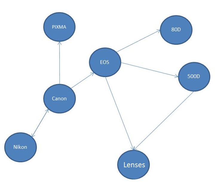
 |
| Example of a bipartite graph from list data |
On the left side of this bipartite graph are the so called "candidate terms", the seedset we provide should be a subset of them. The nodes on the right are called the context nodes, they are representing the link between the candidate terms. In the case of the paper, they have crawled the internet for list items and created an edge to a candidate term if it exists in a given list. The neigbours of a context nodes, are the actual list items in this case. In the case of the web, the picture should also contain words that are not digital camera brands, also think about this simple rule: "more data wins". As in every normal graph, you can also weight the edges, for example if you trust the list data from wikipedia more than of craigslist, then you should assign a higher weight the edges between the context nodes and their candidate term nodes.
I have implemented it by a String array and a DoubleMatrix, where the string array is representing the term nodes and the matrix (NxM, where n is the number of entity tokens and m is the number of context nodes) is representing the weight of the edges. In my experience this matrix is always very sparse, even on very small datasets.
Iterative Similarity Aggregation (the algorithm)
Time to describe the algorithm, now we know how we represented the data.
It is rather simply to explain and I don't know why they complicated it so much in their paper.
There are three main methods, first the relevance score computation, the method that filters out newly top ranked items and at last the ranking function.
The relevance score computation is working like this:
- Loop over all the terms in your matrix while looping over all terms in your seedset
- Get the column vector of your seed element and the column vector of the candidate term
- Measure the similarity between both and sum this similarity over all seedset terms, in the paper it is normalized by the length of the seedset, so it is actually the average similarity
What you now get is a vector (length is the number of term nodes you have), and in each index is the average relevance score to the seedset tokens.
Of course you want to pick the highest relevance nodes of this vector, that's where the static thresholding comes in. You pass the algorithm a similarity threshold, this threshold affects how fast the algorithm converges to a certain solution and how much false positives it will have in the end. Of course a higher threshold will yield to less false positives and faster convergence, while the exact opposite will yield to the other extremum. The truth (as always) lies anywhere between, so it is up to you to choose this correctly.
Since the algorithm always converges quite fast, you can experiment with other thresholds and see how it affects your output. Sure we are going to filter by the threshold and get a number of most relevant new candidate nodes.
Now we can enter the main loop and compute the relevance score again for the newly found relevant candidates (this is now called the similarity score). Based on this we are going to rank these two scores with some simple vecor multiplications:
So where does this alpha come from? That is what the paper names as "weighting factor", as you can see it is used to weight the scores. It is mainly used for the convergence of the algorithm, they say, halfing the scores (alpha = 0.5) yields to the best result.
Once we have a ranked scores, we can now filter again by the similarity threshold and get our new candidate terms for the next iteration.
In each iteration we do:
- Compute similarity score by newly found candidate terms (in the beginning this is the seed set)
- Rank the calculated similarity score against the newly found candidate terms
- Apply the static threshold and get new candidate terms
Until it converges: by means the relevant tokens does not change their order anymore- they are equal. Note that you can also equalize on their ranks, I haven't tried it yet but it should converge also quite fast.
At the end you can now optain your expanded set by getting the candidate terms from the last iteration.
Results
Since I'm working in the e-commerce industry, I wanted to try it out to find similar camera brands like in the paper. It works, but it has very noisy result, partly because the algorithm is just iterative and not parallelized thus I can't work on huge datasets and partly because I had no real clean dataset.
But it really worked, I seeded "Canon" and "Olympus" and got all the other camera brands, sadly a few lenses as well.
On colors there are some similar behaviours, I seeded "blue", "red" and "yellow". Funnyly the most relevant token was "X" and "XS", by means that especially t-shirt products have the color in their name. It became very noise afterwards, found Ronaldo jerseys and other fancy clothes, but a bunch of new colors also.
The paper mentions a really nice trick for it: using the internet!
They have collected millions of list items from websites and let the algorithm run, in my opinion in every machine learning algorithm more data wins. The noise on small dataset will be vanished by the sheer size of the data. So I can very much think that they got really good result.
Parallelization strategy
The easiest way to parallelize this is using BSP and Apache Hama (in my opinion).
Let me tell you why:
- Algorithm is strongly iterative
- Needs communication between a master and the slaves
Here is my strategy to implement this in BSP:
- The bipartite graph is split among the tasks, partitioned by the term nodes
- A slave only partially computes the similarity between the seed tokens and the candidate terms
- A master will be used to put all the similarities back into a single vector, rank it and distribute the newly expanded set again as well as checking convergence.
This is pretty much work, so I guess the follow-up post will take a few weeks. But I promise, I will code this algorithm!
So thank you very much for reading, you can find my sequential code on github, as well as the testcase: